REW, or Room EQ Wizard, is a free software that allows you to measure and analyze the acoustics of a room (typically, a studio).
Although the software is relatively easy to use, you still need to understand how to utilize the various analysis graphs it offers. Especially if your goal is to use it to define the acoustic treatment solutions you will choose.
That’s why I’m offering you this tutorial on using REW. Once you’ve read it, you will know:
- what equipment you need;
- how to take a measurement using the software;
- how to analyze this measurement based on the most useful graphs.
The goal is not to rewrite the manual by detailing every feature, but rather to give you the tools to analyze your (home) studio’s acoustics effectively.
Acoustic Measurement Equipment
Nothing too complicated in terms of equipment.
You will of course need a microphone, but not just any microphone: you need a mic that offers the flattest frequency response possible, so as not to skew the results.
We’re talking about a “measurement microphone.”
Fortunately, you don’t need to spend a fortune: Behringer makes a very good one for around sixty euros. It’s the ECM8000, which I highly recommend because its quality is more than sufficient for this type of application.

Compare the price of the ECM 8000 at: Thomann – Woodbrass – Amazon
You will then need to connect this microphone to an audio interface, which you probably already have in your studio. If not, feel free to check out my article on USB interfaces.
Don’t forget to activate phantom power, as the ECM8000 needs it to operate.
Finally, you will of course need to install the REW software — Room EQ Wizard. You can find the latest version on the official website, under Downloads:
Then all you have to do is launch it, and you’ll be ready to measure the acoustics of your room! 🙂
Set Up the Microphone
Taking the time to position the microphone is very important to ensure that the measurements it produces will be the best possible.
Install it so that it is at head level and exactly the same distance from each of your monitoring speakers (ideally, to the millimeter). If your speakers are well positioned, this shouldn’t pose too many problems.
As for the angle of the microphone relative to the floor, the manufacturer sometimes recommends a specific configuration, but this topic generates a lot of discussion, and it seems that no one has an absolute answer.
In general, if you point the microphone towards the speakers (thus in a horizontal position), it means you will measure the sound from the speakers. If you point it towards the ceiling, you will instead measure the response of the entire room, which corresponds much better to what we want to do.
I therefore advise you to position your microphone vertically.
Note that this choice is not necessarily very important, in the sense that you will primarily compare your measurements before and after treatment. What is important, rather, is that between two measurements the microphone is exactly in the same position and oriented the same way.
Calibrate Your Equipment
Before taking your measurements, it may be useful to calibrate your equipment — or more precisely, to calibrate the REW software to the interface and microphone you are using.
This step is not essential, since once again your measurement work will be done comparatively, before and after installing your acoustic treatment. So if your equipment generates small errors, they will appear in all measurements and will not pose any issues for analysis.
But hey, if you have a few minutes, this calibration step will allow for more accurate results, so you might as well do it properly.
Calibrate your interface
Click on the “Preferences” menu, then select the “Preferences” option (yes, indeed).
A window like this will appear:

Then follow these steps:
- Connect an output (Line Out) of your audio interface to an input (Line In) to create a loop. Indeed, to calibrate the audio interface, we will measure its reaction “in a closed circuit”.
- Select the corresponding inputs/outputs in the “Output” and “Input” fields

Click on the “Calibrate” button
- Click twice on the “Next” button at the bottom of the window
- A sine wave is then generated, but you will not hear it as it is sent from the output to the input you selected.
Adjust the output level so that the level indicators of the “Out” and “In” columns are roughly balanced, as shown in the image to the right. - When the levels are identical or nearly so, click on “Next”.
- Your sound card is then ready to be calibrated. Click on “Next”.
- A new window appears and the measurement is performed automatically.
- Click on the “Make Cal…” button and save the calibration file you generated.

And there you go 🙂
Note: you can optionally skip this step, especially if you are in a home studio context: the measurement results without interface calibration will remain very correct! 🙂
Calibrate your microphone
Similarly, REW allows you to calibrate your microphone via the “Mic/Meter” tab in the “Preferences” panel.
To do this, simply load the calibration file you have.
Note that some microphones, including the Behringer ECM8000, do not come with calibration files. In this case, do not load a file from elsewhere: a calibration file is specific to a particular microphone, not to a model.
Take the measurement
Once the interface and/or your microphone are calibrated, you can finally take a measurement by clicking the “Measure” button in the REW interface.
A window appears allowing you to set a number of things:
- Strat Freq & End Freq (Start and End Frequencies): generally, start at 20 Hz and end at 20 kHz, to cover the entire range of audible frequencies. Tightening this range of values will not be useful because, later, when displaying the data, it will be possible to filter out the data you do not want to see.
- Level: -12 dBFS will be just fine
- Length (Length in samples): the default value of 256k will work perfectly
- Sweeps (Number of frequency range sweeps): 1 will be sufficient at first. Doing several would maximize the signal-to-noise ratio by adding them together.

Then there’s the choice of output. On this point, I strongly advise you to take both an overall measurement (Left+Right) as well as a measurement for each monitoring speaker, and thus to alternately choose the “Left” and “Right” options depending on whether you want to use the left or right speaker.
Why?
You need to distinguish the situation of the bass vs. the situation of the mids and highs.
In the low frequencies, let’s say below 250/300 Hz, sound is less directional. Therefore, at our listening point, we will perceive a sound that is a sum of the sound from the left speaker and the sound from the right speaker. Measuring both speakers at the same time is therefore a good idea.
For the mid and high frequencies, approximately above 250/300 Hz, it is very different: our right ear only partially receives the sound from the left speaker, as it is blocked by our head. Thus, if we measure a sum of the left + right speakers, we risk missing room problems (because that is indeed what we are measuring at the base: the acoustics of the room).
Moreover, still for the mid and high frequencies, measuring the speakers separately will allow you to avoid potential phase issues if your microphone is slightly closer to one speaker than the other.
Finally, the room’s response to one speaker will always be slightly different from that of another speaker, so it is better not to mix the measurements too much…
Before taking any measurements, make sure to wear earplugs for safety: depending on your settings, the volume can be very loud.
Note that you can use the Delay setting to delay the start of the measurement by a few seconds, giving you time to exit the room, for example.
Now use the “Check Levels” button to generate a test signal and adjust the volume of your speakers accordingly until the software indicates “Level OK”.
You can then click on “Start Measuring” to perform the measurement! 🙂
The Frequency Curve
It is time to analyze your results, starting with the “SPL & Phase” tab which simply displays the frequency response curve.
What is it about?
You can visualize, for the entire frequency range covered during the measurement, the sound level that has been measured.
By default, the graph will look something like this:

As you can see, it is a bit difficult to read, especially when we go to the high frequencies. To solve this problem, feel free to apply a “smoothing”, that is to say, a smoothing, using the options in the “Graph” menu in the menu bar at the top of the software.
In REW, a number of smoothings are available, from octave to 1/48 octave. To keep the data sufficiently accurate, stick to the lightest smoothing, namely 1/48 octave. Otherwise, some useful information might disappear:

It’s better, isn’t it?

Which scale to choose?
To facilitate analysis, feel free to click on the “Limits” button at the top right of the graph and choose your own scale:
- Left and Right control the frequency display. You can thus display only the low frequencies if you want to focus on modal resonances.
- Top and Bottom control the sound level range. To make reading easier, I recommend choosing a level range from the level of your highest measurement down to a point about -50 dB lower.
For example, if your highest measurement is around 80 dB, choose a Top at 80 dB and a Bottom at 30 dB.
What do we see on this graph?
Even if this is the graph that will probably speak to you the most if you are used to using equalizers or frequency graphs, it is unfortunately the least useful for acoustic treatment.
However, it is possible to fairly easily identify the room modes in the low frequencies, which will appear as peaks or abnormal dips, as shown in the following diagram:

Since no room or studio is perfect, you will never achieve a perfectly flat curve. However, you can tell yourself that a difference of 10 dB between the maximum and minimum value of your graph indicates a room that is fairly well balanced in frequencies. At least, for a home studio.
The ETC Curve
Click on the “Filtered IR” tab (IR = Impulse Response) and use the checkboxes in the legend to display only the curve called “Envelope (ETC)”.
What is it?
ETC stands for “Energy Time Curve” — in other words, the curve represents variations in energy (volume) over time.
Again, the graph may not look very nice, but that’s not necessarily a big deal. If you really want to smooth the curve, you can click the “Controls” button at the top right of the graph and adjust the “ETC Smoothing (ms)” parameter. Values around 0.1 ms work very well.
You then get something like this:
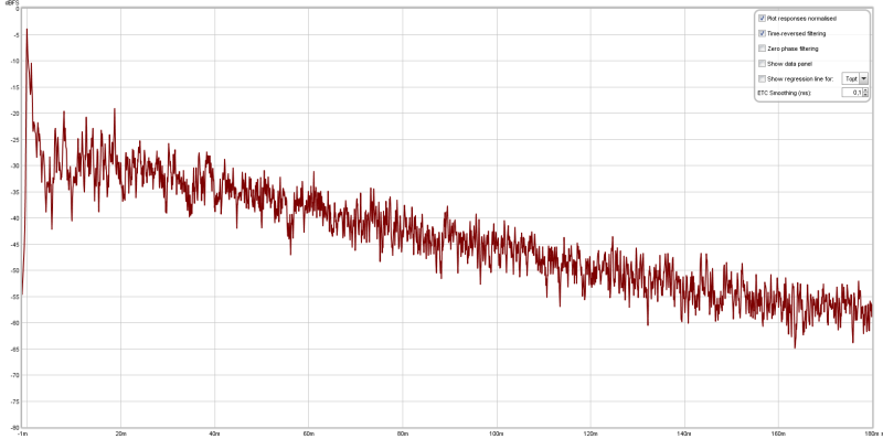
Which scale to choose?
I know, for now this curve is not very informative. But it is useful to look at it on an appropriate scale.
First of all, you need to ask yourself what you are looking at. The first big peak, located at 0 ms, is the speaker’s response. It is the direct sound — therefore normally the first and the loudest — that you hear.
The other peaks are the reflections around you.
First, we know that our brain has difficulty distinguishing between a sound and its reflection if they are spaced less than 100 ms (approximately). The horizontal, temporal scale we will choose will therefore be between 0 and 100 ms.
Vertically, we can choose, for example, a range of values between 0 and -50 or -60 dB. The idea is that reflections at -50 dBFS relative to the initial sound are negligible.
Reminder: to enter these values, use the “Limits” button at the top right of the graph and click “Apply Settings”. Note that the settings are in seconds; for 100 ms, you should enter 0.1 s.
Analyzing the curve
Once these settings are made, it is possible to analyze what is wrong with the curve.
First of all, it is of course preferable that no reflection is as strong as the base signal. So make sure that all reflections are at least -20 dBFS from the original signal. Especially in the first 40-50 milliseconds.
Next, the decrease in the signal should be smooth, avoiding having a peak higher than the previous peak. In practice, this will not be easy, but try to optimize your acoustic treatment with this in mind and install absorbing panels at the first reflection points.
To go further, Room EQ Wizard allows you to filter data by frequency band, via the “Controls” menu (gear icon). I strongly advise you to do this, as some problems may become clearer this way!
A little math
Here’s a tip.
When you see an abnormal peak, you can guess the wall or object (your desk…) that generated it by doing a little calculation.
Let’s say you see a reflection that stands out at 20 ms. The original signal is at 0 ms.
So there are 20 milliseconds between the two, which is 0.02 seconds.
The formula is as follows:
Distance = Speed x Time
The Speed being the speed of sound (on average 340 m/s), we can perform the calculation:
D = 340 * 0.02 = 6.8 m
The reflected signal has therefore traveled 6.8 meters more than the distance between the speakers and the measurement microphone.
This gives you an indication of the position of the object or wall that generated the reflection.
To make this calculation, feel free to use the mini-calculator below:
A duration of milliseconds corresponds to a distance of meter(s).
const ETCcalculator = document.querySelector(‘#ETCdistance’);
ETCcalculator.addEventListener(‘input’, (event) => {
document.getElementById(“ETCresult”).value = document.getElementById(“ETCdistance”).value * 340 / 1000
});
The RT60 / Topt Curve
Now click on the RT60 tab and uncheck all the boxes in the legend except for the one corresponding to the “Topt” curve.
What is it?
Four curves displaying a reverberation time (decay time in English) can be displayed, with octave or third-octave smoothing (via the Controls button):
- RT60 — the time taken for the sound to drop to -60 dB relative to the initial measurement;
- RT30 — the same, at -30 dB;
- EDT — the same, at -10 dB;
- Topt — a proprietary algorithm from REW that adapts very well to small rooms and works similarly to the others.
If you are trying to acoustically treat a home studio, you will probably lean towards this last option.
And here is the result:

Which scale to choose?
The scale is less important here, but I advise you not to use a too large vertical scale that would compress the curve. In other words, if all your values are below 1 second, there is no point in displaying values above that.
In terms of horizontal scale, namely the frequencies, you can usually keep the entire spectrum because the curve is very simple and thus very readable.
Analyzing the curve
I really like this graph because it allows you to see in a “macro” way the effect of the added acoustic treatment. If you install some absorbing panels, you will immediately see the effect on the high frequencies.
It is very telling.
In short, if you use this curve to analyze the effectiveness of your panels or your bass traps, there are two things that you should ideally find:
- a decay time or reverberation time of less than 0.3 seconds across the entire frequency spectrum;
- a variation of less than 10% between two adjacent frequency bands. Indeed, the curve will never be completely flat but it is important that it is sufficiently balanced.
If these conditions are not met, you will likely need to adjust your acoustic treatment accordingly.
The waterfall
Now click on the “Waterfall” tab.
There is nothing there, which is normal: you need to generate the graph by clicking the “Generate” button at the bottom left of the window.
What is it about?
Simply put, this 3D visualization shows the evolution of energy (sound level) over time for the entire frequency spectrum.
It’s a bit like displaying, side by side, the measured frequency curve every “X” milliseconds.
You can thus see, for example, if your lows around 100 Hz resonate longer than all the other frequencies – or conversely if they are absent (due to modal resonances).
Which scale to choose?
In short, by default the graph is hard to read and quite bland:

You will therefore need to adjust the scale and set up the graph to have something usable.
To facilitate reading, I recommend cutting the waterfall graph 50 decibels below the maximum measured value.
To do this, click on the “Limits” button at the top right and indicate:
- at Top, the maximum measured value (visible on the graph, no need to be very precise, round to the nearest ten)
- at Bottom, the same value from which you will subtract 50 dB
Like this:

Then, for the horizontal scale (Left and Right), it depends on what you want to display:
- either you want to focus on the modal resonances of your room, thus on the lows, and in that case you will display a waterfall between about 20 and 300 Hz
- or you want to have a global overview of how your room/studio resonates, and in that case you will select the entire recorded frequency band
Finally, the time scale (depth on the graph) needs to be appropriate. Click on the “Controls” button and adjust the “Time Range (ms)”.
If we take the values mentioned for the Topt/RT60 curve, we think that ideally, reflections should be below 0.3 seconds, or 300 milliseconds. You can therefore choose this value, or one just above (400-500 ms). It doesn’t matter if the graph is slightly truncated: on the contrary, you will better identify the problems.
Analyzing the curve
By reading my text about the scale, and as we reach the end of this article, I think you are starting to get an idea of what can be done.
Thanks to the waterfall graph, it is possible to easily identify modal resonances. Indeed, in the lows, certain frequencies will resonate for far too long, while others will clearly disappear.

In the image above, this is precisely the case: the frequency 113 Hz is completely absent from the start of the measurement! 🙂
Similarly, if you have placed too many absorbing panels and your highs are too muffled, you will see on this waterfall that the high frequencies are more retracted compared to the mid or low frequencies.
This graph proves to be quite useful, as it provides a global view of the room’s acoustics but also allows for detailed analysis of the measurements.
In conclusion
There you go, with all this you should be able to start measuring the acoustics of your (home) studio, or your hi-fi listening room effectively.
What is important to realize is that it is only by analyzing all of these curves that you will have a true understanding of your room. Therefore, it is impossible to only look at one to go faster: each has its utility…
…the goal being of course to install appropriate treatment! 🙂
Just to go further and if you haven’t already done so: feel free to take a look at my guide on acoustic treatment to avoid the most common mistakes.
And to go even further, I recommend the SawUp training on acoustic treatment, which is just THE best French-speaking training on the subject, for anyone looking to seriously approach the acoustic treatment of their (home) studio or audiophile room.